
Population and representative samples
When it comes to mining, we aim to extract the economic portion of a population (the portion that makes a profit). We do not know our full population. Instead, we rely on a miniscule subset of the population (the samples) to make our decisions. If we are to make reasonable decisions, the samples we rely on must represent the total population.
What makes a sample set representative? In statistical terms, this means the samples we collect of the population provide a fair indication of how the population behaves.
A histogram is a useful plot for understanding the population and for measuring of the population distribution. A histogram is a plot of the count of data points within successive intervals (see an example histogram for copper in Figure 1). This bar chart provides a summary of typical spread of grades in the data set.
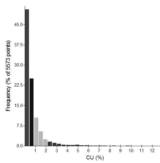
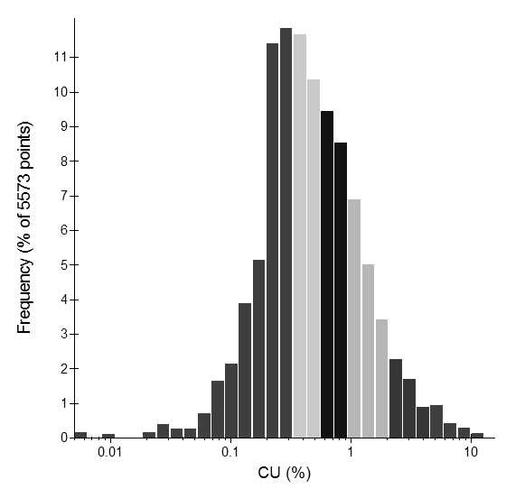
When a data set has a positive skew, most of the sample values are low grade with a small percentage of more extreme high grades. This means most of the samples occur within a few intervals of the histogram (see the left hand bars of the histogram in Figure 1). A useful option is to change the intervals for the histogram. The easiest way to do this is to apply a log-transform to the data. A log-transform maintains the data order, so the same low grades samples on a normal scale are low grades on a log-scale, and the highest sample on a normal scale is still the highest sample on the log-scale. Figure 2 is a log-scale histogram of the data presented in Figure 1. A log-transformation effectively magnifies the lower grade end of the distribution and contracts the higher grade scale.
A sample histogram is a representative reflection of the population histogram when it accurately reflects the total population (Figure 3).

A good way to ensure a representative data set is to have fair coverage of the population (no bias introduced by clustered drilling) and even sampling within each geologically controlled population (as best as can be achieved – often samples are collected over variable lengths to represent the various geological units or population controls).
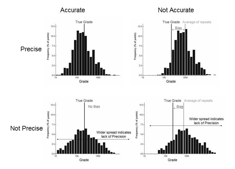
In addition, for a sample to be representative the difference between the sample value we obtain and the true value should be as close as possible. If we take numerous repeat samples at the identical location, the difference between them should be small and the average of all of them should be as close to the true value as possible. This means the samples are precise (small overall error) and accurate (close to the true value). The consistent difference between the average of the repeat samples and the true value is called a bias.
Precision, accuracy and bias
In reality, data collection errors lead to a mismatch between what we sample and the population we are trying to represent. This difference can occur in the following ways:
· Precision describes our ability to be specific about a grade – the number of decimal places we report describes our ability to be precise. Precision is measured by comparing repeat samples.
· Accuracy describes how well the average of the repeat samples targets the true (but unknown) grade.
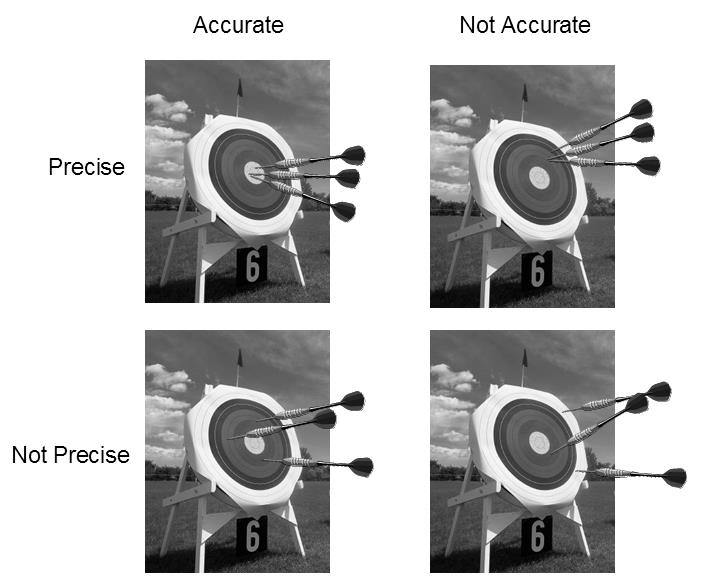
Bias is the measure of the systematic difference between the average of our repeat samples and the true grade.
In statistical terms, the histograms of the repeat samples either reflect the true unknown value or not according to a shift in the average away from the true mean (a bias), or a wider than acceptable spread (lack of precision) as described in Figure 5.
In reality, samples invariably incur a degree of imprecision and inaccuracy. We need to ensure that through proper sampling practices the errors incurred are as small as possible.
Samples and lots
Samples are collected at different volumes – consider the difference between the volumes of 1m of RC chips compared with the volume of the pulp that is eventually analysed in the laboratory. Pierre Gy describes these differences as the “lot” or the “sample”, where the sample is the volume ultimately analysed for grade, while the lot is the volume of material collected for sampling.

Other examples of lots are: blasthole cone, diamond core, development face chips and stockpiles. Examples of samples are half diamond core, riffle split sample, mill pulp and fire assay sample.
Activity
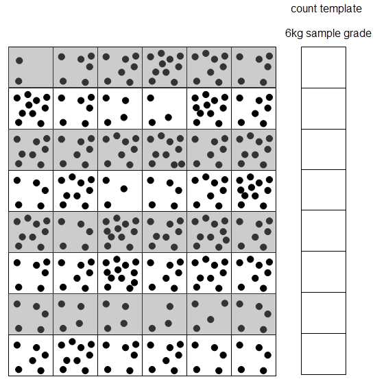
Consider a 48 kg lot that contains precious grains. We are interested in the number of grains per kg. The lot is divided into 48 one-kilogram samples. 1. Count the grains per kilogram within each sample (record in count template).

2. Calculate the overall average of the samples . This is the grade of the lot.
3. How well does each sample reflect the grade of the lot? To answer this question, plot a histogram of the sample grades.
Highlight the lot grade on the histogram. Compare the sample grades to the lot grade.
Calculate the variance and standard deviation.
What does this tell you about the precision of the samples?
4. Suppose we take bigger samples, say 6kg samples. How precise will these samples be? To answer this, calculate each 6kg sample’s grade as grains per kilogram.
Calculate the overall average. Calculate the standard deviation. How does this compare to the standard deviation of the 1kg samples?
5. Suppose there is a problem with your counting apparatus. For each 1kg sample, a grain is lost. With this adjustment, recalculate the true grade of the lot.

Recalculate the standard deviation of the samples and plot the histogram of the problem data.

What do you observe?